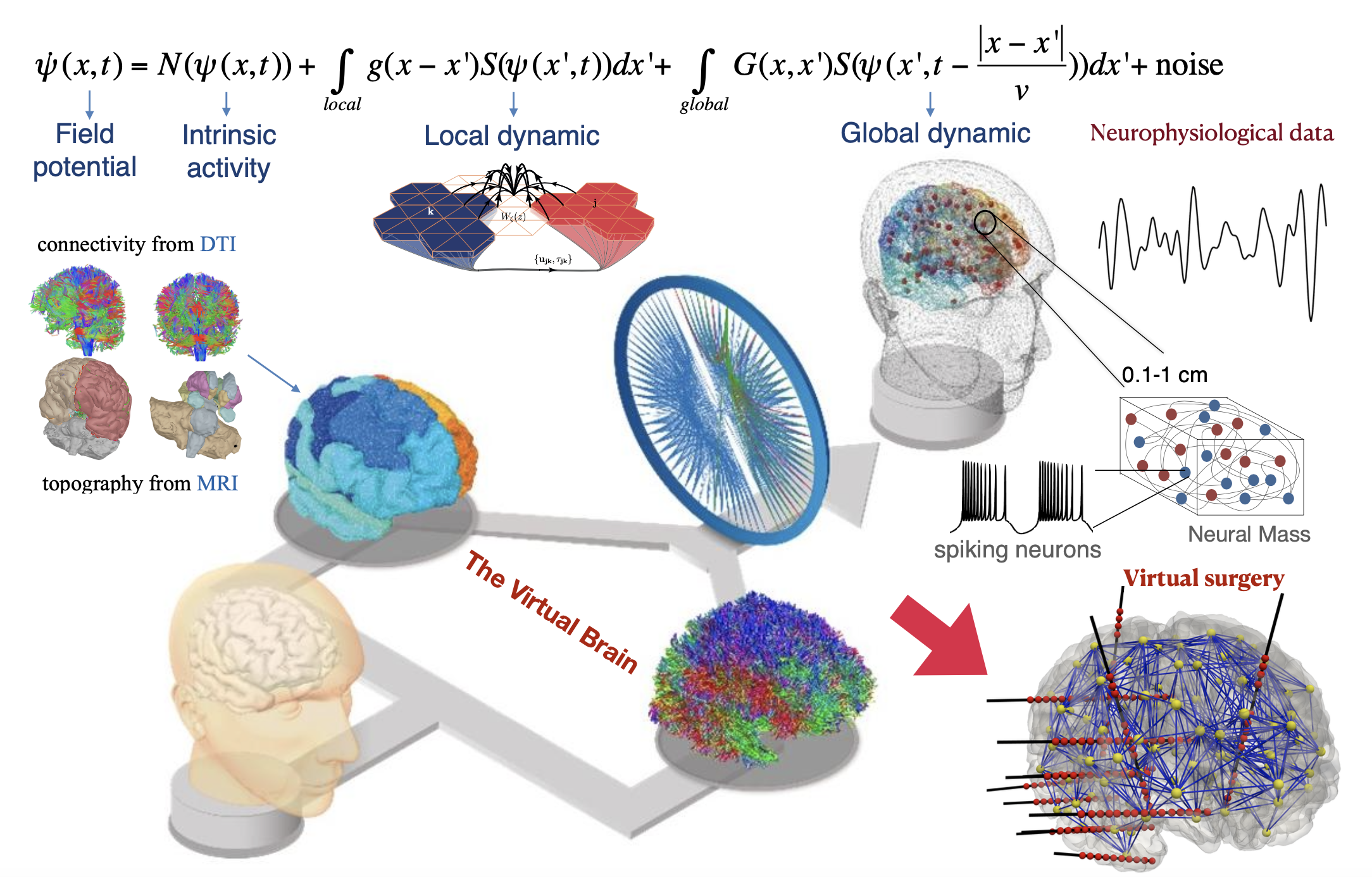
The treatment of brain disorders faces two main challenges. First, most clinical decisions are validated via population-based trials, often neglecting individual variability. Second, the lack of a theory of brain (dys)function makes mechanism-based approaches very difficult, which contributes to our slow pace in delivering effective treatments for epilepsy and Alzheimer’s disease as prototypical examples. My research program focuses on development of strategies and technologies to advance personalized and mechanism-based approaches. Specifically, I wish to: (1) predict individual responses to treatments, (2) reduce comorbidities often associated with treatment, and (3) inform clinical decision-making. To achieve this, we can rely on Virtual Brain Modelling and Bayesian inference. The former integrates structural and functional data into mechanistic models to simulate individual brain activity in silico. The latter refines the simulations to enhance personalization, leveraging ML/AI algorithms. The tools will be flexible enough to adapt to brain scales and conditions, making them essential in scenarios where experiments are prohibitive (e.g., new electrode implantation).
Contact me for a possible collaboration!
As evidence accumulates in support of the predictive power of virtual brain models (such as BVEP), and software development used in clinical trials (EPINOV, the world’s first clinical trial in Epilepsy using virtual brain model), they are likely to inform changes in clinical practice in the near future. The aim is to infer the parameters of these models by fitting them to various neurophysiological data, in order to identify the origin of brain (dys)function in biological space. The prospects for predictive personalized medicine in a digital environment to optimize drug dosage or intervention strategies, with preventive and therapeutic targets, will be offered in clouds (EBRAINS).
Scientific background on Mote Carlo simulations:
1. What is Monte Carlo used for?
Monte Carlo simulations, also known as the Monte Carlo methods are a broad class of stochastic algorithms that rely on repeated random sampling, which are mainly used in three problem classes: inverse problem (optimization), numerical integration, and generating draws from a probability distribution to estimate the possible outcomes of an uncertain event (see Fig. 2). For instance, to understand the impact of risk and uncertainty in prediction and forecasting models, Monte Carlo simulations are used to estimate the probability of different outcomes in a process that cannot easily be predicted due to the intervention of random variables. Monte Carlo simulations let us to analyze all the possible outcomes of the decisions and assess the impact of risk, allowing for better decision making. Furthermore, mathematical formulation of many physical and biological systems contains parameters that are typically unknown or known only with large uncertainty. The uncertainty associated with unknown parameters translates into an uncertainty in model prediction, consequently, in hypothesis evaluation, which itself significantly affects decision-making processes. Moreover, dynamic models involve latent variables, which cannot be measured directly, hence requiring inference from latent space (abstract representation of a real-world system) to understand the emergent dynamics of a complex system. Bayesian inference is a principled method for statistical inference that updates the prior belief about a hypothesis with new evidence from observed data, thus naturally characterizing uncertainty over unknown quantities.
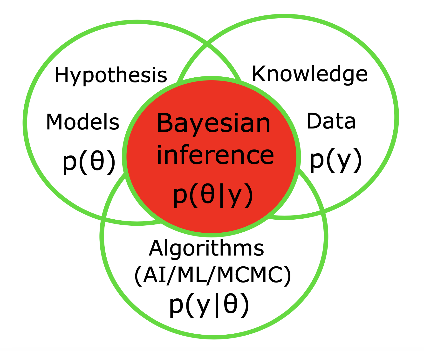
Computational modeling allows us to simulate real-world systems, thus learning about the data generation process, making predictions on unseen data, and justifying the hypotheses. By running various simulations with different inputs, we can gain insight into different potential outcomes, thus providing evidence to support or refute hypotheses regarding the effects and mechanisms of a certain phenomenon. In contrast to forward modeling, which is a top-down approach, model inversion (e.g., simulation-based inference) is a bottom-up strategy that infers hidden causes from observed effects. Having various source of information and system spatio-temporal scales, the Bayesian inference provides a unified framework to merge the models, data, prior information and algorithms to reach reliable scientific conclusion. This approach allows for the incorporation of uncertainty and prior knowledge in the hypothesis testing process (such as anatomical data, MRI lesion, the target of stimulation or evidence from previous trials on drug efficacy, etc), which is important for understanding the underlying causes of diseases, hence to improve the predictions for better decision-making processes at the individual and group levels.
2. What do we need to perform Monte Carlo simulations?
Monte Carlo methods to perform Bayesian inference (inverse problem) involves the following steps:
3. How to choose an algorithm to carry out an inverse problem with Monte Carlo?
The performance of algorithms for inverse problems with Monte Carlo simulations is task-dependent, and there is no uniformly best algorithm across different tasks. This indicate the need for domain expertise and service offerings. In the following, the state-of-the-art algorithms as the bridge the gap between data, models, and decision makers is briefly discussed.
4. Who uses Monte Carlo Simulations?
Many companies use Monte Carlo simulations as an important part of their decision-making process. General Motors, Procter & Gamble, Pfizer, Bristol-Myers Squibb, and Eli Lilly use Monte Carlo simulations to estimate both the average return and the risk factor of new products. Easy to use, integrated with open source, comprehensive and flexible, Webdemo, Cloud computing, graphical interface for user (in uploading data and loading results), with free trial, are the important features that industrial partners attempt to offer. High fidelity simulations, AI acceleration without sacrificing accuracy is the trend for all applications that use Monte Carlo simulations.
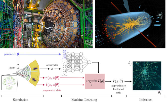
Fig. 4) Particle physics processes are usually modelled with complex Monte-Carlo simulations of the hard process, parton shower, and detector interactions. These simulators typically do not admit a tractable likelihood function: given a (potentially high-dimensional) set of observables, it is usually not possible to calculate the probability of these observables for some model parameters. Particle physicists usually tackle this problem of “likelihood-free inference” by hand-picking a few “good” observables or summary statistics and filling histograms of them. But this conventional approach discards the information in all other observables and often does not scale well to high-dimensional problems. Simulation-based-inference (SBI) with state-of-the-art deep learning algorithms called Normalizing-Flows can solve these problems.
Credit: CERN. See: MadMiner
Amortized Bayesian inference on specific EEG features during general anesthesia:
The past decade has explored new frontiers of research into the effects of general anesthesia. Although general anesthesia is commonly used in medical care for patients undergoing surgery, its precise underlying mechanisms remain to be elucidated. There are, however, several hypotheses that have been advanced to explain how general anesthesia occurs [1-2].
Despite a global reduction in neuronal activity under general anesthesia, specific regions in the brain have been shown to have markedly increased/decreased activity [3-4]. The cortex, thalamus, and other subcortical structures appear to be involved in changes of arousal during general anesthesia [4-5]. However, the evidence in the literature has not conclusively established whether anesthetics target the cortex directly or indirectly by Thalamo-cortical (TC) disruption, hypothalamic inhibition, microtubule interaction, or a combination of all three. Recent progress in consciousness research has determined the involvement of the TC network on several key features of consciousness [6-13]. TC circuits play a key role in the generation of brain rhythmic activities and hence, to explain specific features observed experimentally both in frontal and occipital electrodes during general anesthesia, such as induced slow oscillations, paradoxical excitation, anteriorization, and beta buzz activity. Although anesthetics directly bind to specific receptors [14-15], general anesthesia induced by various anesthetics is accompanied by some common features in EEG rhythms [1-2]. However, the mechanisms responsible for these characteristic changes are still unknown. It has been shown that TC neural mass models (set of nonlinear delay differential equations) are able to produce different anesthetics induced EEG features [10-12], but their parameter estimation is a necessary task to accurately explain the experimental observations for better understanding of the neural mechanisms underlying general anesthesia [16-17].
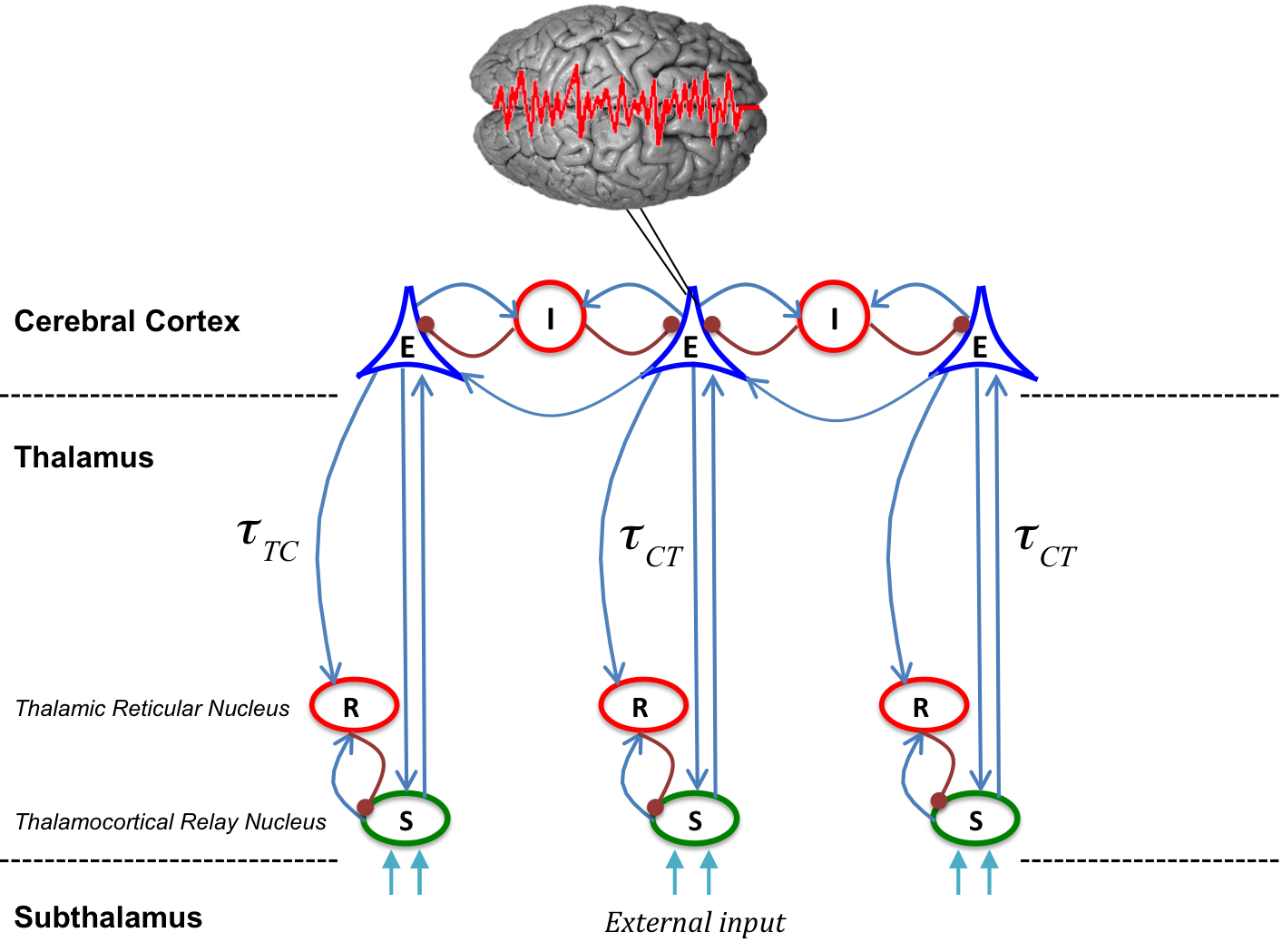
Fig. 5) The model consists of four types of neural populations, namely, cortical excitatory (E) and inhibitory neurons (I), thalamo-cortical relay (S), and thalamic reticular neurons (R). The blue arrows show excitatory connections while the red connections with filled circle ends indicate inhibitory connections. The connections from cortex to thalamus is associated with the time delay τ_TC, whereas the latency for signals in reverse direction is τ_CT. The external input to the system originating from subthalamic areas is considered as a non-specific input to relay neurons.
Parameter estimation of the next generation neural mass models:
A key question in neuroscience is how brain function organization arises from the collective dynamics of networks of spiking neurons. The mean-field theories provide insights into macroscopic states of large neuronal networks in terms of the collective firing activity of the neurons, or the firing rate [39]. The next generation of neural mass equations can exactly describe all possible macroscopic dynamical states of the spiking networks, including states of synchronous activity [40-41]. Coupling a set of exact macroscopic equations for the networks of spiking excitatory and inhibitory neurons, then it is necessary to estimate the effective coupling between biophysically relevant macroscopic quantities, the firing rate and the mean membrane potential, which together govern the evolution of the spiking neural network. The firing-rate equations (FREs) are generally derived through heuristic arguments that rely on the underlying spiking activity of the neurons being asynchronous and hence uncorrelated. As such, firing-rate descriptions are not sufficient to describe network states involving some degree of spike synchronization. Hence, the lack of firing-rate descriptions for synchronous states limits the range of applicability of mean-field theories to investigate neuronal dynamics. FREs for networks of heterogeneous, all-to-all coupled quadratic integrate-and-fire (QIF) neurons, can be derived analytically as exact in the thermodynamic limit, i.e., for large numbers of neurons [40]. More interestingly, a set of FREs is able to fully describe the macroscopic response of an infinite number of QIF neurons to time varying stimuli (up to finite-size effects), such as a step function or sinusoidal forcing [40], which can be the target of fitting for inferring the neural population responses to the brain stimulation.
Bayesian inference on generative model of whole brain dynamics:
Despite the widespread use of connectome-based predictive modeling for revealing the mechanisms underlying dynamics of large-scale brain networks, the advanced Bayesian algorithms to overcome the inference difficulties have received no attention in this context. Using personalized whole-brain modelling approach, the subject specific anatomical information can be combined with the mean-field models of local neuronal activity to mimic the individual's spatio-temporal brain activity at the macroscopic scale [50]. However, model prediction and validation from a complex system characterizing the macroscopic dynamics of the population of neurons is challenging due to high-dimensionality of parameter-space as well as the intrinsic non-linear dynamics of neural population models [51-52]. In this project, we will use the mean-field models of neural activity exhibiting saddle-node and Hopf bifurcations, which is combined by anatomical connectivity obtained from non-invasive imaging techniques to infer and validate the model parameters against the multimodal neuroimaging data. Then, we will employ the recently developed sampling algorithms in probabilistic programming tools to systematically predict the mechanisms by which the functional brain imaging data are generated. Our previous results have indicated that the automatic self-tuning Bayesian algorithms are able to accurately estimate the brain region specific parameter (for 84-400 coupled nonlinear SDEs), while the convergence diagnostics and posterior behaviour analysis validate the reliability of the estimations [24-25]. Here, an ambitious idea is that one may infer a closed-form of the function governing the system dynamics over both the system (hidden) states and the transition function rather than only the model parameters [51-52]. Moreover, we will investigate the efficiency of the model reparameterization and hierarchical structure in prior information using Bayesian inversion of the nonlinear state space equations. The Bayesian framework enables us to integrate the individual's anatomical data in the prior information to establish an appropriate patient-specific strategy for estimating macroscopic dynamic of large-scale brain network models with the associated uncertainty translated in posterior distribution [25]. This approach can improve out-of-sample prediction accuracy for identification of pathological areas in the brain [26].
Dynamic Causal Modeling (DCM) for inferring whole-brain effective connectivity:
DCM [53] is a well-established framework for analyzing neuroimaging modalities (such as fMRI, MEG, and EEG) by neural mass models where inferences can be made about the coupling among brain regions (effective connectivity) to infer how the changes in neuronal activity of brain regions are caused by activity in the other regions through the modulation in the latent coupling. Although DCM can be used to model and track the changes in excitatory–inhibitory balance from functional neuroimaging modalities [54], this approach has been mainly employed for single neural mass model (i.e., small number of cortical sources), while the non-linear ordinary differential equation representing the neural mass model is approximated by its linearization around a fixed point of the system. Using automatic Bayesian inference in PPL tools such as Stan/PyMC3 [42-43], we will be able to scale DCM to efficiently infer whole-brain effective connectivity [55]. However, with such inference from coarse-grained and low temporal resolution time series like BOLD signals, the non-identifiability (degeneracy) issue is ubiquitous in model configuration space. There are different ways to deal with non- identifiability in the Bayesian inference such as using shrinkage methods (e.g., the spike-and-slab or horseshoe prior [21]) for sparse estimation, or adding the more level information in prior/ likelihood function, as well as data augmentation to break degeneracies and multicollinearity in the model configuration space.
Bayesian inference on heterogeneity in complex systems:
Disentangling the heterogeneity of brain (for instance, brain regional variation in aging, Alzheimer's disease, and other cognitive impairment) is a challenging problem in systems neuroscience [56]. The brain functional connectivity dynamics can be modelled by complex systems (such as coupled generic Hopf oscillators [57]) to find diagnostics/biomarkers for degenerative cognitive disorders. However, parameter estimation of complex systems to explore the synchronized states of coupled oscillators is an ill-posed inverse problem (the emergent synchronization frequency of the oscillators is independent of the natural frequency distribution). In some instances, we can reparametrize the model configuration space that transforms the poorly informed parameters into parameters that are less coupled, and hence better identified from the measurement process. A careful manifold reparameterization will reorganize the model configurations consistent with the data generating processes into geometries that better match the capabilities of the algorithm and actually facilitate accurate estimation. Transforming the system configuration from time-space to (spectral) frequency-domain will give the sampler a decent chance of fully quantifying the posterior distribution, thus to accurately infer the heterogeneity in the model parameters. Taking this approach, we will then establish biomarkers based on training a deep neural network on functional connectivity (FC, [58]), and/or functional connectivity dynamic (FCD, [59]) as the key data features in emergent complex neural dynamics to diagnose the various spatiotemporal patterns observed over cognitive impairment period.
Degeneracy in systems neuroscience:
Degeneracy [60] is ultimately a question of information, in particular how much information we have about the chosen parameters that coordinate the model configuration space. If a realized likelihood function or posterior density function is degenerate then we need to incorporate more information into our inferences or alternatively, reparameterize the model configuration space.
It is well-known that gradient-free sampling algorithms such as Metropolis-Hastings, Gibbs sampling and slice-sampling generally fail to explore the parameter space efficiently when applied to large-scale inverse problems as often encountered in the application of whole-brain imaging for clinical diagnoses. In particular, the traditional MCMC mix poorly in high-dimensional parameter spaces involving correlated variables [21]. In contrast, gradient-based algorithms such as Hamiltonian Monte Carlo (HMC) although computationally expensive, they are far superior to gradient-free sampling algorithms in terms of the number of independent samples produced per unit computational time [22]. This class of sampling algorithms provides efficient convergence and exploration of parameter space even in very high-dimensional spaces that may exhibit strong correlations. Nevertheless, the efficiency of gradient-based sampling methods such as HMC is highly sensitive to the user-specified algorithm parameters. In particular, the performance of HMC is highly sensitive to the step size and the number of steps in leapfrog integrator for updating the position and momentum variables in Hamiltonian dynamic simulation. If the number of steps in the leapfrog integrator is chosen too small, then HMC exhibits an undesirable random walk behaviour similar to Metropolis-Hastings algorithm, and thus algorithm poorly explores the parameter space. If the number of leapfrog steps is chosen too large, the associated Hamiltonian trajectories may loop back to a neighbourhood of the initial state, and the algorithm wastes computation efforts. NUTS algorithm [23] extends HMC with adaptive tuning of both the step size and the number of steps in leapfrog integration to sample efficiently from complex posterior distributions.
References:
[1] Zeisel J, Bennett K, Fleming R. World Alzheimer Report 2020: Design, dignity, dementia: Dementia-related design and the built environment.

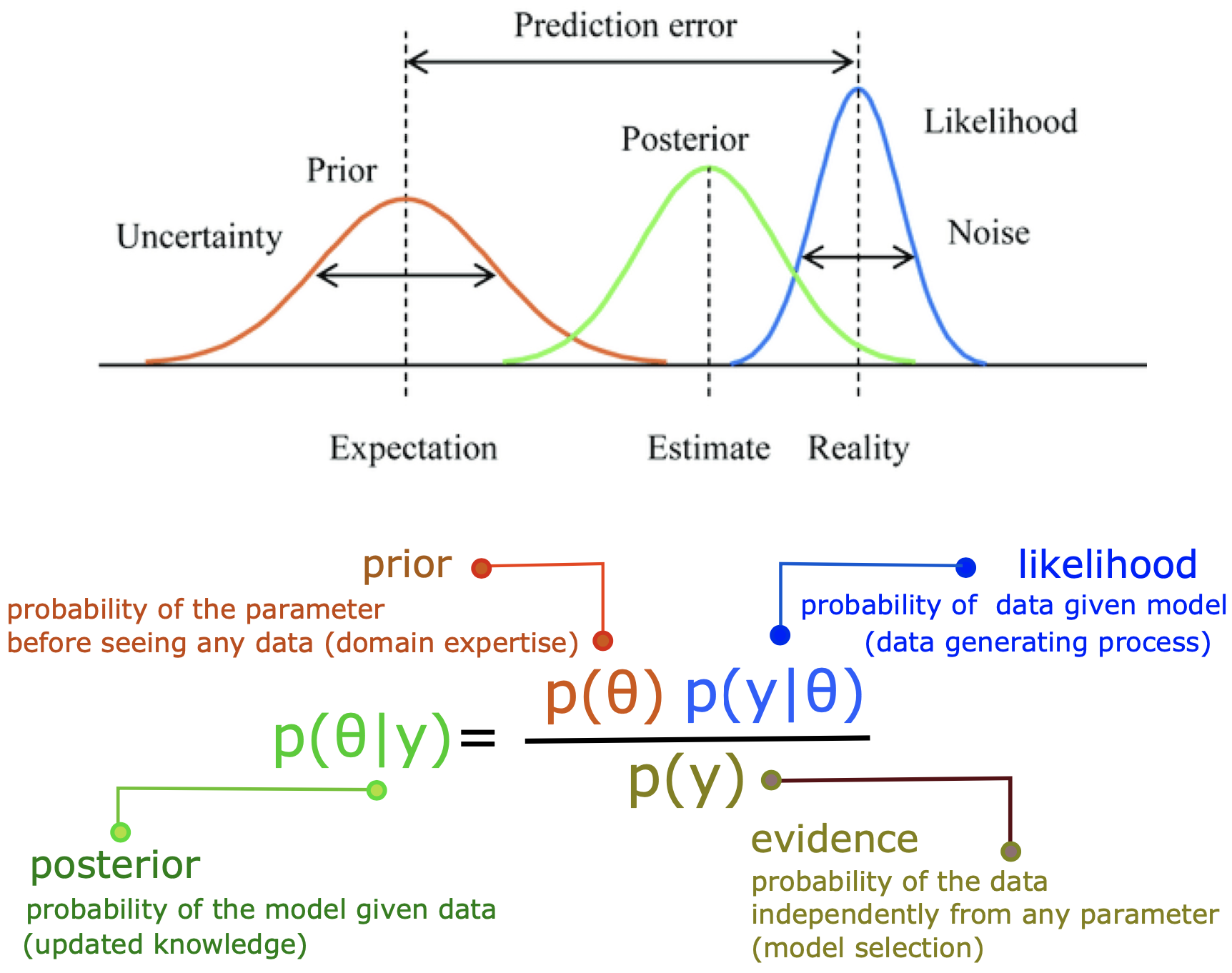
The Bayesian framework (see Fig 3.) offers a powerful approach to deal with model uncertainty in parameter estimation, and a principled method for model prediction with a broad range of applications including clinical hypothesis testing. The Bayes theorem states that the posterior probability of θ can be calculated proportional to the product of the prior probability of θ and the data likelihood, i.e., Prob(θ|y) ∝ Prob(θ) Prob(y|θ).
Bayesian techniques infer the distribution of unknown parameters (the posteriors) of the underlying data generating process given only observed responses and prior information about the underlying generative process. Moreover, Bayesian framework allows us to integrate patient-specific information in the prior knowledge as well as the uncertainty regarding the system organization (neural circuits) in the model likelihood function to improve out-of-sample prediction accuracy.
Broadly speaking, given a set of experimental data and a particular mathematical model, the aim of parameter estimation is to identify the unknown parameters with associated confidence intervals (uncertainties) of the estimates. In general, there are two broad classes of approaches for solving parameter estimation problems: the Frequentist inference and Bayesian estimation. Compared to its frequentist counterpart, the Bayesian framework has several unique advantages, and its incorporation into parameter estimation, hypothesis testing, and clinical trial design is occurring more frequently. For instance, considering the treatment effect in a clinical trial, which is the unknown parameter of interest, the frequentist framework assumes that parameter (denoted by θ) is fixed, yet unknown but through clinical trials, we can collect data (denoted by y) to inform the parameter. Hence, the inference on the treatment effect can be made by evaluating the conditional probability of data given parameter, Prob(y|θ), where the data are considered to be random and the parameter is fixed. Conversely, the Bayesian framework is intrinsically hierarchical by assuming that the data (y) are fixed and the unknown parameter (θ) is random, thus the inference is made by computing the conditional probability of parameter given data (not conditioned on the design experiment), i.e., Prob (θ|y). Despite the usefulness and proven success of frequentist approach in model evaluation and clinical trials, the frequentist framework suffers from some major deficiencies. Most notably, frequentist inference on the parameter of interest, θ, is made indirectly as it calculates Prob(y|θ) and not Prob(θ|y), as Bayesian inference does. In other words, the frequentist approach requires a stronger assumption that observations are identical and independent, underestimate the variability of the parameter of interest, whereas Bayesian setting allows for the incorporation of a priori information and sequential learning to refine the hypotheses, providing the uncertainty of the random variable to make decision based upon the variance of the distribution.
In the context of clinical trials, using Frequentist approach, prior information (based on clinical evidence from previous trials) is utilized only in the design of a trial but not in the analysis of the data. On the other hand, Bayesian approach provides a formal mathematical framework to combine prior information with available information at the design stage, during the conduct of the experiments, and at the data analysis stage.
1) Analyzing and better understanding the data to extract relevant and low-dimensional features, which can be modeled/fitted.
2) A Bayesian model of the data generating process, i.e., a statistical model where the probability is used to represent both the uncertainty regarding the output and the uncertainty regarding the input (i.e., parameters or latent states) of the model. In contrast to black box methods, this step requires knowledge about the model components such as hierarchical dependencies in probabilistic model, identifying both dependent variables to be predicted and independent variables that will drive the prediction, as well as specifying prior probability distribution on all unobserved variables/parameters.
3) Implementation of the Bayesian models in a computer program to sample from the posterior. The efficiency of sampling critically depends on both data and model (the calculation of the likelihood function). Running Monte Carlo methods typically requires a large number of model evaluations, which demand powerful computer resources and high-performance computing. In high dimensional parameter spaces, the higher the number of samples on Monte Carlo methods, the better is the approximation, subsequently, they have a large demand on computational resources.
The use of cloud computing for parallel computing offers some advantages over conventional clusters: high accessibility, scalability and pay per usage. Facility Hubs can provide access to supercomputing
network and cloud computing for data storage, analysis, simulation, and running Monte Carlo algorithms in parallel.
4) Algorithmic convergence, diagnostics, and validation. Once the model is fitted, it is necessary to assess the convergence to the “true” stationary solutions that help ensure high accuracy and quality decision making. The convergence diagnostics specific to the used algorithm, and posterior behavior analysis (e.g., posterior predictive check), and out-of-sample prediction are necessary to validate the reliability of the model estimations.
Markov chain Monte Carlo (MCMC) is a non-parametric method that requires explicit evaluation of the likelihood function and is asymptotically unbiased to sample from the posterior distribution (through stochastic transformations). However, evaluation of the target distribution can be prohibitive expensive in high-dimensional spaces, often with the rejection of many proposals that impose the search space exploration to converge very slowly. The sensitivity of MCMC methods to the user-specified algorithm parameters is also a common issue for efficient sampling. While gradient-based algorithms such as Hamiltonian Monte Carlo (HMC) are well suited to sampling from high-dimensional distributions, it may take many evaluations of the log-probability of the target distribution and the gradient for the chain to converge, in particular, when the geometry of the target distribution is highly non-linear. In the presence of parameter degeneracy, sophisticated reparameterization techniques changing local geometry of the posterior is required to improve the efficiency of Monte Carlo sampling.
Of the alternatives, Variational Inference (VI) turns the Bayesian inference into an optimization problem, which typically results in much faster computation than MCMC methods. While the mean-field VI fails to capture dependencies and multi-modality in the true posterior, the derivation of the full-rank VI requires a major model-specific work on defining a variational family appropriate to the probabilistic model, computing the corresponding objective function, computing gradients, and running a gradient-based optimization algorithm. The probabilistic programming languages (PPLs) solve these issues for automatic inference, by providing self-tuning algorithms and automatic differentiation methods, in which probabilistic models can be specified relatively easily and inference for these models is performed automatically. In particular, Stan, Turing, and PyMC3 are high-level statistical modeling tools for Bayesian inference and probabilistic machine learning. However, the performance of sampling/optimization algorithms in PPLs can be sensitive to the form of model parameterization.
For high-dimensional and complex models, when standard methodologies cannot be applied due to analytic or computational difficulties to calculate the likelihood function, one can use the simulation-based inference (SBI). The core of this methodology only requires forward-simulations from the computer programming of a parametric stochastic simulator (also referred to as generative model), rather than model-specific analytic calculation or exact evaluation of likelihood function. This approach was used for the discovery of the Higgs boson (see Fig. 4.), where a gigantic simulator generates the data but a few parameters needed to be to estimated. The classical method for SBI is known as Approximate Bayesian Computation (ABC). In practice, ABC-related methods suffer from the curse of dimensionality, scale poorly to high-dimensional and non-Gaussian data, and their performance depends critically on the choice of discrepancy measure (summary statistics), and the tolerance level which determines whether the measures are sufficiently similar. Normalizing-Flows (NFs) are a novel family of generative models that convert a simple distribution into any target complex distribution, where both sampling and density evaluation can be efficient and exact. In this approach, a simple base probability distribution (e.g., a standard normal) is transformed into a more complex (potentially multi-modal) target distribution through a sequence of invertible mapping (implemented by deep neural network). These neural density estimators form a family of methods that estimate conditional densities with the aid of neural networks, designed to estimate the full posterior distribution, dealing with degeneracy and potential multi-modalities.
IBM Cloud Functions can also assist in Monte Carlo Simulations. IBM Cloud Functions is a serverless functions-as-a-service platform that executes code in response to incoming events. Read more about how to conduct a Monte Carlo Simulations using IBM tooling, here.
The Spectrum Symphony offering on IBM Cloud is used to create all the necessary resources and to configure the HPC cluster for evaluating the Monte Carlo workload. IBM Cloud Functions can provide a phenomenal boost to a Monte Carlo simulations, which is considered to be an important High-Performance Computing workload. IBM® SPSS® Statistics is a powerful statistical software platform. It offers a user-friendly interface and a robust set of features that lets your organization quickly extract actionable insights from your data. Advanced statistical procedures help ensure high accuracy and quality decision making.
At CERN, the production of Monte Carlo simulations is an important step to investigate several aspects of the experimental apparatus, minimizing the instrumental errors due to target acceptance, geometry and the errors deriving from the analysis cuts. Geant4 is a platform for the simulation of the passage of particles through matter using Monte Carlo methods. Geant4 includes facilities for handling geometry, tracking, detector response, run management, visualization and user interface. For many physics simulations, this means less time needs to be spent on the low level details, and researchers can start immediately on the more important aspects of the simulation. A team of researchers at CERN, SURFsara, and Intel, are investigating the use of deep learning engines for fast simulation. This work is being carried out as part of Intel’s long-standing collaboration with CERN through CERN openlab. CERN openlab is a public-private partnership, founded in 2001, which works to help accelerate innovation in Information and Communications Technology (ICT). Today, Intel and CERN are working together on a broad range of investigations, from hardware evaluation to HPC and AI.
A service on Monte Carlo simulations is required to include all four steps as data analysis, model selection, programming and cloud computing, as well as the validation, which it is highly challenging to integrate all aforementioned steps in a pipeline. The current services are offered as only either cloud computing or software production. The full service in particular model selection, state-of-the-art algorithms, and validation is currently lacking. In the context of neuroscience, we have extensive experience in working with various neural models and dynamical systems with the state-of the-art algorithms (implemented in PPLs or by deep neural networks) to guide clinician and researchers and deploy this service.
Broadly speaking, given a set of experimental data and a particular mathematical model, the aim of parameter estimation is to identify the unknown parameters with associated confidence intervals (uncertainties) of the estimates. In general, there are two broad classes of approaches for solving parameter estimation problems: the Frequentist inference and Bayesian estimation [18]. Compared to its frequentist counterpart, the Bayesian framework has several unique advantages, and its incorporation into parameter estimation, hypothesis testing, and clinical trial design is occurring more frequently [19]. For instance, considering the treatment effect in a clinical trial, which is the unknown parameter of interest, the frequentist framework assumes that parameter (denoted by θ) is fixed, yet unknown but through clinical trials, we can collect data (denoted by y) to inform the parameter. Hence, the inference on the treatment effect can be made by evaluating the conditional probability of data given parameter, Prob(y|θ), where the data are considered to be random and the parameter is fixed. Conversely, the Bayesian framework is intrinsically hierarchical by assuming that the data (y) are fixed and the unknown parameter (θ) is random, thus the inference is made by computing the conditional probability of parameter given data (not conditioned on the design experiment), i.e., Prob (θ|y). Despite the usefulness and proven success of frequentist approach in model evaluation and clinical trials, the frequentist framework suffers from some major deficiencies. Most notably, frequentist inference on the parameter of interest, θ, is made indirectly as it calculates Prob(y|θ) and not Prob(θ|y), as Bayesian inference does. In other words, the frequentist approach requires a stronger assumption that observations are identical and independent, underestimate the variability of the parameter of interest, whereas Bayesian setting allows for the incorporation of a priori information and sequential learning to refine the hypotheses, providing the uncertainty of the random variable to make decision based upon the variance of the distribution. In-depth comparisons between the frequentist and Bayesian approaches can be found in the literature [17-20].
The Bayesian framework offers a powerful approach to deal with model uncertainty in parameter estimation, and a principled method for model prediction with a broad range of applications including clinical hypothesis testing. The Bayes theorem states that the posterior probability of θ can be calculated proportional to the product of the prior probability of θ and the data likelihood, i.e., Prob(θ|y) ∝ Prob(θ) Prob(y|θ). Bayesian techniques infer the distribution of unknown parameters (the posteriors) of the underlying data generating process given only observed responses and prior information about the underlying generative process [21]. Moreover, Bayesian framework allows us to integrate patient-specific information in the prior knowledge as well as the uncertainty regarding the system organization (neural circuits) in the model likelihood function to improve out-of-sample prediction accuracy [24].
Monte Carlo Markov Chain (MCMC, [19]) methods are able to calculate the unnormalized posterior densities. MCMC has the advantage of being non-parametric and asymptotically exact in the limit of long/infinite runs. However, MCMC-based sampling of posterior distributions, which converge to the desired target distribution for large enough sample size, is a challenging task due to the large curvature in the typical set or non-linear correlations between parameters in high-dimensional parameter spaces [22]. Although an efficient Bayesian inversion requires painstaking hyperparameter tuning, the novel methods in artificial intelligence can efficiently provide the posterior distribution and the relation between model parameters for different observations of a subject without having to re-run inference. Based on simulating artificial dataset conditioned on the sampled parameters, several likelihood-free inference methods such as Normalizing Flows [26-27] and VAEs [28-29] efficiently perform inference, in particular when likelihood computations are prohibitively expensive. Despite the theoretical and technological advances, practical implications of these algorithms in a Bayesian inference paradigm with information-theoretic measures for model selection and clinical hypothesis testing remain to be explored. The main advantage of these deep learning algorithms, compared to the traditional MCMC and VI, is amortized approximating the intractable likelihood function based on the defined data features while they are able to estimate the multimodality in posterior distributions.
Using amortized Bayesian inference, the aim is to train deep neural networks such as Normalizing Flows or VAEs on a TC neural mass model to fit EEG patterns according to the specific features observed experimentally during general anesthesia. These novel deep learning models rely on the idea that the data generated by a model can be parametrized by some variables that will generate some specific characteristics of a given data point, allowing both feature learning and tractable marginal likelihood estimation [31-32].
Normalizing Flows are the next generation deep learning algorithms in a chain of invertible transformations on an initial distribution, which produce tractable distributions where both sampling and density evaluation can be efficient and exact [26-27]. In Normalizing Flows, we aim to map simple distributions (easy to sample and evaluate densities) to complex ones (learned via data). We take a simple probability distribution (uniform or Gaussian), take a sample from it and then transform the sample. This is equivalent to change of variables in probability distributions and, it can result in a very complex probability density function of the transformed variable. “Normalizing” means that the change of variables gives a normalized density after applying an invertible transformation. “Flow” means that the invertible transformations can be composed with each other to create more complex invertible transformations.
A Variational Autoencoder (VAE) provides a probabilistic manner for describing an observation in latent space [28-29]. One of the key ideas behind VAEs is that instead of trying to construct a latent space (space of latent variables) explicitly and to sample from it in order to find samples that could actually generate proper outputs (as close as possible to target distribution). The VAEs can be viewed as two coupled, but independently parameterized models: the encoder or recognition model, and the decoder or generative model. These two models support each other. The recognition model delivers to the generative model an approximation to its posterior over latent random variables, which it needs to update its parameters inside an iteration of expectation maximization learning. Reversely, the generative model is a scaffolding of sorts for the recognition model to learn meaningful representations of the data, including possibly class-labels. The recognition model is the approximate inverse of the generative model according to Bayes rule.
Of the alternatives, the mean-field variant of variational inference (VI, [32]) lets us to approximate a high-dimensional posterior with a simpler Gaussian distribution by solving an optimization problem (minimizing the KL divergence between actual and approximate distributions). This approach has been successfully used in various models and is able to scale for very large (hundreds-thousands) dimensions. However, the classical derivation of VI requires a major model-specific work on defining a variational family appropriate to the probabilistic model, computing the corresponding objective function, computing gradients, and running a gradient-based optimization algorithm. Although the Automatic Differentiation Variational Inference (ADVI [33]) solves these issues automatically, it may get stuck in local minima during gradient descent optimization while its mean-field variant is unable to cover all the modes of the multi-modal posterior densities. Consequently, in the case of multimodal posterior distribution, the information is discarded in the favour of highest mode and it biases the model selection task.
In a Bayesian framework, for the purposes of model comparison, selection and averaging, the out-of-sample model predictive accuracy (i.e., the measure of model's ability in new data prediction) is needed following the fitting of a probabilistic model to the observed data [34-35]. For instance, different configurations of the underlying generative process and observation including variation in parameters and data features can be fitted, and then compared by out-of-sample prediction accuracy to determine the best performing among a set of candidates. This procedure can similarly be performed for clinical hypothesis testing to explore the sensitivity and specificity of the potential mechanisms in model predictions based on new data, hence for selection of the best balance between complexity and accuracy. Several information-based criteria have been proposed for measuring the model predictive accuracy (e.g., AIC/BIC, and KL divergence or free energy) [36]. However, the fully Bayesian criteria (e.g., WAIC, or leave-one-out cross-validation [37]) which are based on the whole posterior distribution rather than a point estimate or a simple approximation to normal distribution, have received little attention in this context. By definition, the classical information criteria such as AIC/BIC are independent of prior information (essentially by MLE assuming uniform prior), in which if the penalty term (number of parameters and observed data) is similar across different candidates, it becomes infeasible to determine the best among a set of hypotheses [24-25]. In contrast, WAIC and LOO cross-validation are reliable and robust techniques (fully Bayesian), enabling us to integrate our prior information (based on the clinical expertise) about the model parameters to improve the model's ability in new data prediction. Currently used in a clinical trial (EPINOV, RHU project), we have recently developed a fully Bayesian framework to infer the spatial map of epileptogenicity in a personalized large-scale brain model of epilepsy spread [24]. The influence of prior information on out-of-sample model prediction evaluated by fully Bayesian criteria (such as WAIC and LOO) to select the best clinical hypothesis was also investigated in detail. We showed that an informative prior knowledge based the dynamical system properties merged with the clinical expertise is required to provide significant evidence in favour of the best clinical hypothesis [25, 51-52].
Regarding the data features for training the deep neural networks, using Wiener-Khinchin theorem [38], we can analytically calculate the spectral power of a stochastic system (to avoid the computational burden due to numerical integration of the model equations) that dramatically alleviate the computational cost of model inversion due to the variability in observations. Following the model reparameterization in frequency domain, then the artificial neural network can learn the spectral features and following the training, they can exactly reproduce the propofol-induced changes in the EEG power spectrum across subjects. During sedation before achieving full general anaesthesia, the observed specific changes in electroencephalographic (EEG) rhythms comprise increased activity in the δ− (0.5−4 Hz) and α− (8−13 Hz) frequency bands over the frontal region, but increased δ− and decreased α−activity over the occipital region [6-10]. An increased GABAergic inhibition onto TC cells results in an α− resonance that is reinforced by reciprocal corticothalamic feedback, and hence leads to the emergence of frontal α−activity. This frontal enhancement and occipital attenuation of α−activity is commonly termed anteriorization [6]. Another prominent feature in the EEG of some patients is the emergence of a strong power peak in the β-frequency band, which moves to the α-frequency band while increasing the anaesthetic concentration. This feature is called the beta-buzz [16]. These features can be sufficiently informative for the convergence of Normalizing Flows or VAEs. Using these novel machine-learning techniques in the spirit of Bayesian inference, then we are able to reliably evaluate different hypotheses regarding the sufficient changes/causality in level in transfer function properties and synaptic parameters and/or in feedback loops of excitatory-inhibitory populations for the generation of spectral EEG characteristics. Moreover, maximizing the marginal likelihood function using deep neural networks based on dynamical properties of the system such as the fixed points or the bifurcation diagram can significantly improve training performance. By inferring the causality in TC system, we can provide evidence for different hypotheses such as if the thalamus itself constitutes the primary focus of anesthetic modulation, or if changes that appear within it are secondary effects from other brain regions. Finally, performing a group analysis using cross-validation and hypothesis testing (by fully Bayesian model comparison metric, WAIC), we can then elucidate the effects of anesthetics on the level of excitation-inhibition as well as the feedback loops in the TC system, and likely on the time scale of the system for a cohort of subjects. Understanding the brain organization and the role of its subnetworks associated with the transition from awake condition to anesthetic-induced state will provide new insights into the mechanisms of alterations in consciousness, and can lead to novel therapies and anesthetics targeting specific structures.
Although an efficient Bayesian inversion for these neuronal networks requires painstaking model-specific tuning, one can estimate the likelihood function in PPL tools such as Stan [42] and PyMC3 [43] using self-tuning Hamiltonian Monte Carlo sampling algorithms [23]. Probabilistic programming is becoming one of the most active areas of development in the machine learning. The probabilistic programming paradigm featured by the self-tuning sampling algorithms and automatic differentiation provides high-level tools to solve complex inverse problems conditioned on large data set as the observation. Conceptually, probabilistic programming languages (PPLs) are domain-specific languages that describe probabilistic models and the mechanics to perform inference in those models. The power of PPLs relies on combining the inference capabilities of probabilistic methods with the representational power of programming languages and exact automatic differentiation in codes [44]. In a PPL program, assumptions are encoded with prior distributions over the variables of the model. During execution, a PPL will launch an inference procedure to automatically compute the posterior distributions of the parameters of the model based on observed data. PPLs such as Stan/PyMC3 are flexible and high-level tools for Bayesian inference and probabilistic machine learning, which provide the advanced inference algorithms such as NUTS and ADVI, enriched with extensive and reliable diagnostics [42-43]. Stan is the is a state-of-the-art platform for statistical modeling and can be run in different interfaces, whereas PyMC3 provides several MCMC algorithms for model specification directly in native Python code. Although PPLs allow for automatic inference, the performance of these tools can be sensitive to the form of parameterization in model configuration space. An appropriate form of reparameterization in the probabilistic models to improve the inference efficiency of system dynamics (governed by a set of nonlinear stochastic differential equations) remains a challenging problem. Recently, we have demonstrated the efficiency of the transformed non-centered parameters in comparison to centered form of parameterization for inverting the nonlinear state-space equations [24]. However, despite the efficiency of PPLs, the likelihood function can become computationally expensive for a large number of coupled neural populations to calculate by MCMC. In such cases, we can alternatively run Normalizing Flows [26-27] or VAEs [28-29] to approximate the likelihood function by deep neural networks, without the sensitivity to the tolerance level in the accepted/rejected parameter setting based on low dimensional summary statistic. Despite the theoretical and technological advances in this area, their practical implications for nonparametric Bayesian inference in systems neuroscience have remained to be explored. Using these approaches, then we can investigate the changes in the neural couplings and/or the causality as well as the level of excitation-inhibition from collected data emerging from spiking neurons.
NUTS can manage moderately degenerate posterior density functions by consuming more computational resources. In such cases, the NUTS complains loudly by the need for smaller discretization time, or step size, a larger number of leapfrog steps, or divergent transition due to high curvatures, the non-compact or discontinuous degeneracies. In the use case of Normalizing Flows or VAEs, the degeneracies lead to non-shrinkage posterior distribution (i.e., no gain through information flow).
The most direct way to reduce degenerate behavior in our inferences is to add more information. In practice, however, repeating the measurement process exactly is often prohibitively expensive if not outright impossible. A powerful alternative to repeating the initial measurement process is to complement it with additional measurement processes that are sensitive to only some phenomenological, environmental, or experimental parameters. This complementary data can then break degeneracies in the likelihood function, allowing the original data to inform the rest of the parameters. Bayesian analyses also benefit from the opportunity to add information through the prior model [25].
For the purpose of inferring the epileptogenic zone (EZ) in the brain, when the brain regions are located far from electrodes (for instance in the right hemisphere for left temporal epilepsy), the regional inference is an ill-posed inverse problem and the EZ is then structurally/practically non-identifiable due to the sparsity of the lead-field matrix in Stereoelectroencephalography (SEEG) recordings [24-25, 51-52]. The complementary data from sodium fMRI imaging, PET, or MEG recording can be integrated in the prior information to reduce the degeneracy by incorporating stronger prior information for model inversion. This approach can demonstrate the importance of multimodal functional neuroimaging in brain model-based prediction. Consequently, due to the high level of information for unobserved data prediction, the fully Bayesian information criteria (e.g., WAIC, [36, 37]) will be able to provide significant evidence in favor of the correct EZ hypothesis. In the case of brain regional inference from resting state data using multi-stable dynamical system to capture functional connectivity observed in BOLD signals, the degeneracy is ubiquitous since an infinite combination of model parameters results in similar emergent dynamics.
Because the particular geometry of a realized likelihood function or posterior density function depends on a chosen parameterization of the model configuration space, so too will our definition of degeneracy. In some instances, we can reparameterize the model configuration space and replace poorly-identified parameters with new parameters that are better suited to the measurement process. A realization that appears degenerate in one parameterization might appear much less degenerate in another. This parameterization dependence, however, also provides an opportunity for moderating degeneracy problems. Weak degeneracy implies that every parameter is strongly informed independently of the others. If some parameters are strongly coupled then we might be able to find a reparameterization that transforms them into parameters that are less coupled, and hence better identified. Although there is no unique universal recipe for model reparameterization, the symmetry breaking, time-scale separation, dynamic mode decomposition, QR factorization or singular value decomposition are potential solutions to decorrelate the linear dependencies between parameters for dealing with degeneracy in sampling from model configuration space.
[2] Deco G, Kringelbach ML, Arnatkeviciute A, Oldham S, Sabaroedin K, Rogasch NC, Aquino KM, Fornito A. Dynamical consequences of regional heterogeneity in the brain’s transcriptional landscape. Science Advances. 2021 Jul 14;7(29):eabf4752.
[3] Frégnac Y. Big data and the industrialization of neuroscience: A safe roadmap for understanding the brain?. Science. 2017 Oct 27;358(6362):470-7.
[4] Park DC, Reuter-Lorenz P. The adaptive brain: aging and neurocognitive scaffolding. Annual review of psychology. 2009;60:173.
[5] Proix T, Bartolomei F, Guye M, Jirsa VK. Individual brain structure and modelling predict seizure propagation. Brain. 2017 Mar 1;140(3):641-54.
[6] Courtiol J, Guye M, Bartolomei F, Petkoski S, Jirsa VK. Dynamical mechanisms of interictal resting-state functional connectivity in epilepsy. Journal of Neuroscience. 2020 Jul 15;40(29):5572-88.
[7] Sanz-Leon P, Knock SA, Spiegler A, Jirsa VK. Mathematical framework for large-scale brain network modeling in The Virtual Brain. Neuroimage. 2015 May 1;111:385-430.
[8] Schirner M, Domide L, Perdikis D, Triebkorn P, Stefanovski L, Pai R, Popa P, Valean B, Palmer J, Langford C, Blickensdörfer A. Brain modelling as a service: the virtual brain on EBRAINS. arXiv preprint arXiv:2102.05888. 2021 Feb 11.
[9] Amunts K, Rowald A, Petkoski S, Sanchez-Vives MV, Axer M, De Bonis G, Pennartz C, Bjaalie J, Brovelli A, Fousek J, Ioannidis Y. The coming decade of digital brain research-A vision for neuroscience at the intersection of technology and computing. Computational and Systems Neuroscience; 2022.
[10] Olmi S, Petkoski S, Guye M, Bartolomei F, Jirsa V. Controlling seizure propagation in large-scale brain networks. PLoS computational biology. 2019 Feb 25;15(2):e1006805.
[11] Sip V, Petkoski S, Hashemi M, Dickscheid T, Amunts K, Jirsa V. Parameter inference on brain network models with unknown node dynamics and spatial heterogeneity. bioRxiv. 2022 Jan 1:2021-09.
[12] Chaudhuri R, Gerçek B, Pandey B, Peyrache A, Fiete I. The intrinsic attractor manifold and population dynamics of a canonical cognitive circuit across waking and sleep. Nature neuroscience. 2019 Sep;22(9):1512-20.
[13] McIntosh AR, Jirsa VK. The hidden repertoire of brain dynamics and dysfunction. Network Neuroscience. 2019 Sep 1;3(4):994-1008.
[14] Fousek J, Rabuffo G, Gudibanda K, Sheheitli H, Jirsa V, Petkoski S. The structured flow on the brain's resting state manifold. bioRxiv. 2022 Jan 1.
[15] Hansen EC, Battaglia D, Spiegler A, Deco G, Jirsa VK. Functional connectivity dynamics: modeling the switching behavior of the resting state. Neuroimage. 2015 Jan 15;105:525-35.
[16] Battaglia D, Boudou T, Hansen EC, Lombardo D, Chettouf S, Daffertshofer A, McIntosh AR, Zimmermann J, Ritter P, Jirsa V. Dynamic Functional Connectivity between order and randomness and its evolution across the human adult lifespan. NeuroImage. 2020 Nov 15;222:117156.
[17] Hashemi M, Vattikonda AN, Sip V, Guye M, Bartolomei F, Woodman MM, Jirsa VK. The Bayesian Virtual Epileptic Patient: A probabilistic framework designed to infer the spatial map of epileptogenicity in a personalized large-scale brain model of epilepsy spread. NeuroImage. 2020 Aug 15;217:116839.
[18] Lavanga M, Stumme J, Yalcinkaya BH, Fousek J, Jockwitz C, Sheheitli H, Bittner N, Hashemi M, Petkoski S, Caspers S, Jirsa V. The virtual aging brain: a model-driven explanation for cognitive decline in older subjects. bioRxiv. 2022 Jan 1.
[19] Berry AS, Shah VD, Baker SL, Vogel JW, O'Neil JP, Janabi M, Schwimmer HD, Marks SM, Jagust WJ. Aging affects dopaminergic neural mechanisms of cognitive flexibility. Journal of Neuroscience. 2016 Dec 14;36(50):12559-69.
[20] Sorrentino P et al. Virtual multiple sclerosis patients (submitted)
[21] Petkoski S, Jirsa VK. Normalizing the brain connectome for communication through synchronization. bioRxiv. 2022 Jan 1:2020-12.
[22] Schöll M, Lockhart SN, Schonhaut DR, O’Neil JP, Janabi M, Ossenkoppele R, Baker SL, Vogel JW, Faria J, Schwimmer HD, Rabinovici GD. PET imaging of tau deposition in the aging human brain. Neuron. 2016 Mar 2;89(5):971-82
[23] Stumme J, Jockwitz C, Hoffstaedter F, Amunts K, Caspers S. Functional network reorganization in older adults: Graph-theoretical analyses of age, cognition and sex. NeuroImage. 2020 Jul 1;214:116756.
[24] Bandyopadhyay A, Bernard C, Jirsa VK, Petkoski S. Mean-field approximation of network of biophysical neurons driven by conductance-based ion exchange.
[25] Yu M, Sporns O, Saykin AJ. The human connectome in Alzheimer disease—relationship to biomarkers and genetics. Nature Reviews Neurology. 2021 Sep;17(9):545-63.
[26] Palop JJ, Mucke L. Amyloid-β–induced neuronal dysfunction in Alzheimer's disease: from synapses toward neural networks. Nature neuroscience. 2010 Jul;13(7):812-8.
[27] Gonçalves PJ, Lueckmann JM, Deistler M, Nonnenmacher M, Öcal K, Bassetto G, Chintaluri C, Podlaski WF, Haddad SA, Vogels TP, Greenberg DS. Training deep neural density estimators to identify mechanistic models of neural dynamics. Elife. 2020 Sep 17;9:e56261.
[28] Hashemi M, Vattikonda AN, Jha J, Sip V, Woodman MM, Bartolomei F, Jirsa V. Simulation-Based Inference for Whole-Brain Network Modeling of Epilepsy using Deep Neural Density Estimators. medRxiv. 2022 Jan 1.